>>> Check out the Ipython Notebook in GitHub
- Intro
The Dataset for ADL (Activities of Daily Living) Recognition with Wrist-worn Accelerometer is a public collection of labelled accelerometer data recordings to be used for the creation and validation of supervised acceleration models of simple ADL.
It can be downloaded from the UCI Machine Learning Repository.
The Dataset is composed of the recordings of 14 simple ADL
(brush_teeth, climb_stairs, comb_hair, descend_stairs, drink_glass,
eat_meat, eat_soup, getup_bed, liedown_bed, pour_water, sitdown_chair,
standup_chair, use_telephone, walk) perfomed by a total of 16
volunteers. Note that 5 of those activities had less than 5 records each (brush_teeth, eat_meat, eat_soup, use_telephone), therefore I removed them from the analysis as they are too few to allow proper features learning.
The data are collected by a single tri-axial accelerometer (x, y, z) attached to the right-wrist of the volunteer, sampled at 32 Hz.
EDIT: In this post, I will try to classify accelerometer's data into their corresponding activity in two ways: [1] extracting a number of features I chose to compute to characterize each record's time series, and [2] leveraging the amazing tsfresh library, which automatically extracts and selects from more than 2000 features specifically designed to summarize time series data. In both cases, I will (A) first extract a number of features characterizing each recorded time series, (B) afterward I will feed all those features to a set of classifiers to see which perform best, and finally (C) I will build an ensemble classifier by stacking those classifiers having best performances.
- I will assess the performance of each classifier using the micro F1-score, a metric which summarizes both the precision and the recall (see explanation below): in fact the F1-score is the harmonic mean between the two, averaged over all classes to be predicted. For this particular multilabel classification task, I will use the "micro" F1-score, a way of getting the average F1-score that takes into account possible unbalances between classes (as it is the case in this dataset, see below)
- A perfect model has an F1-score of 1.
- - Precision: the fraction of true positive examples among the examples that the model classified as positive. In other words, the number of true positives divided by the number of false positives plus true positives.
- Recall: also known as sensitivity, is the fraction of examples classified as positive, among the total number of positive examples. In other words, the number of true positives divided by the number of true positives plus false negatives.
Naif approach
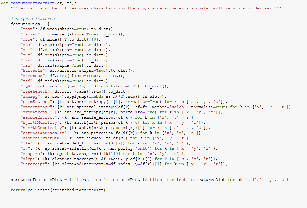
In the first case, I will manually compute, for each time series (x, y, z) of each record, the following features: mean, median, mode, STD, SEM, sum, min, max, kurtosis, skewness, MAD, IQR, line length, energy, permutation entropy, spectral entropy, SVD entropy, sample entropy, Hjorth mobility, Hjorth complexity, Petrosian fractal dimension, Higuchi fractal dimension, Detrended Fluctuation Analysis, coefficient of variation, Shapiro's estimator, slope and intercept.
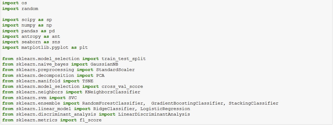
- 1. Import Libraries
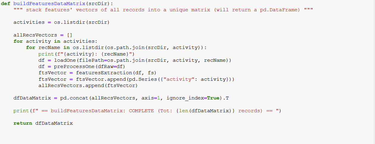
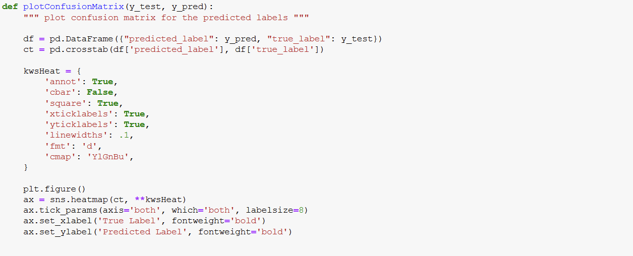
2. Define Helper Functions





3. Define General Variables and print list of recorded human activities


4. Plot four records as example

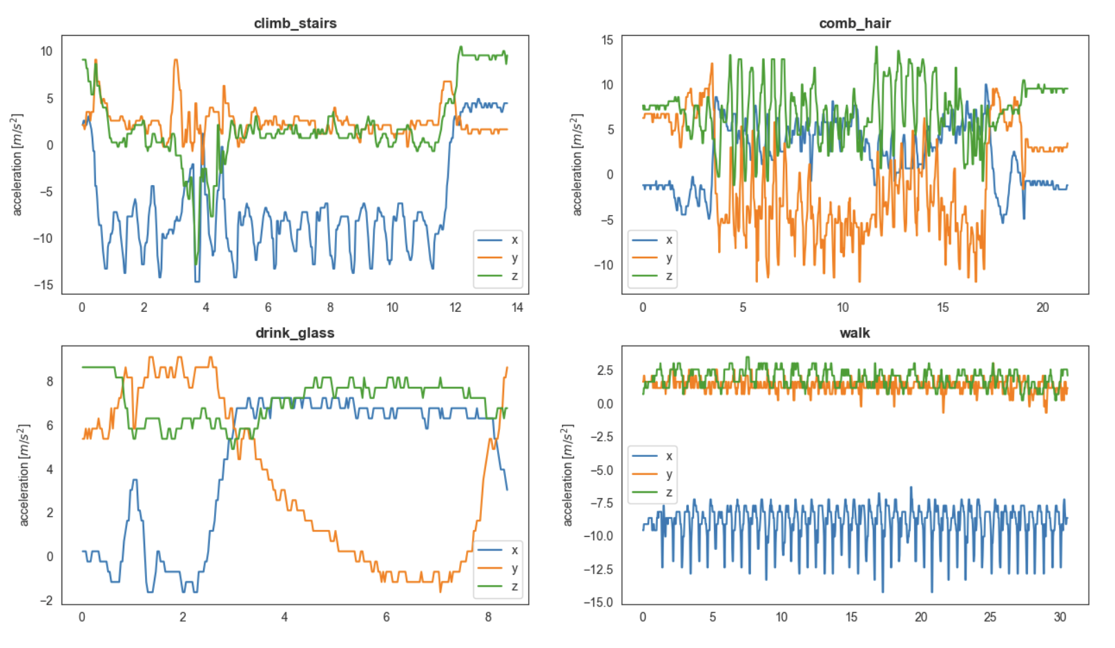
5. Load all time series, extract features, store all in a matrix


From the above list, we can see that we are working with unbalanced classes, therefore we should take this into - that is why we will quantify classification performance using the micro F1-score.
6. Prepare data
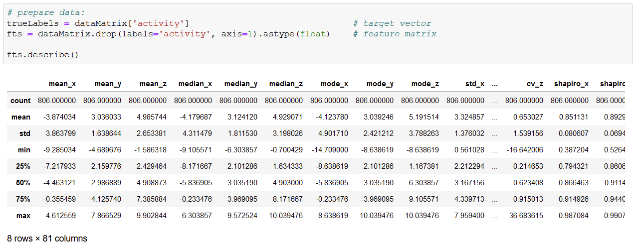
We see that the classifiers will be feed 81 features per record.
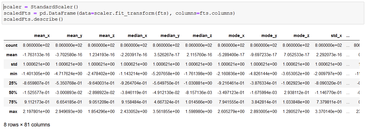
7. Normalize data
8. Plot t-distributed Stochastic Neighbors Embedding plot
t-SNE is a dimensionality reduction algorithm that can be used to map multi-dimensional data into 2 (or 3) dimensions, where observation sharing similar features will tend to stay close, and far from different ones; therefore t-SNE makes possible to get some insights about the relationships between observation and variables.

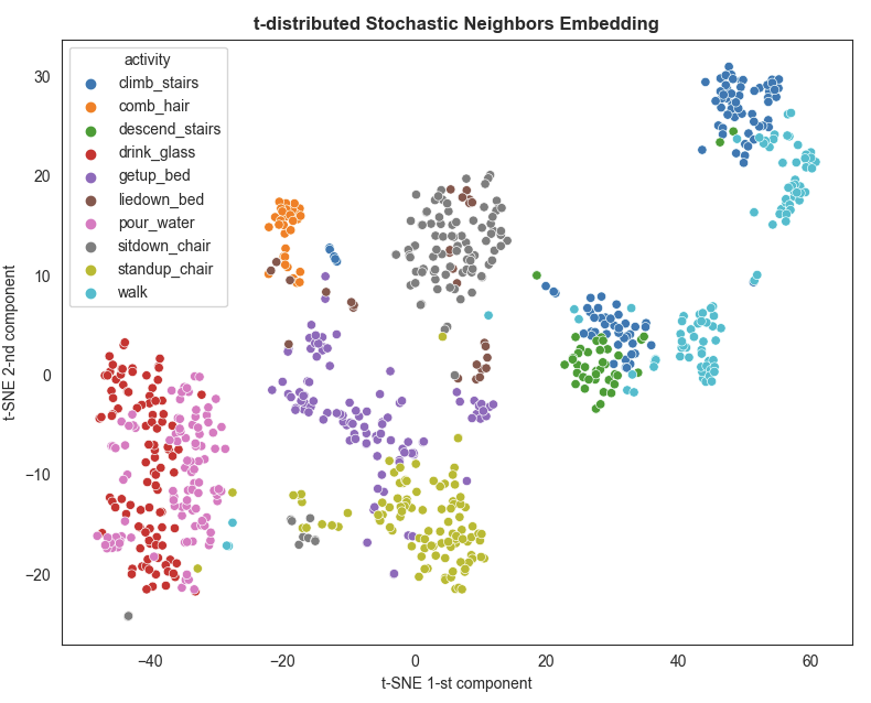
From the above plot, we can appreciate some interesting -even though maybe not so unexpected- things: (a) drink_glass and pour_water tend to be characterized by similar accelerometer's features, (b) there is some kind of cluster regrouping getup_bed, liedown_bed, sitdown_chair and standup_chair, (c) and another "archipelago" composed by climb_stairs, descend_stairs and walk: all this makes kind of sense, isn't it?
However, we also see that those "clusters" are not so precisely separated, therefore we should take this result with caution.
9. Split data into train and test set (stratifying by label as classes are unbalanced)

10. Instantiate list of classifiers

11. Run classification and return F1-score for each classifier

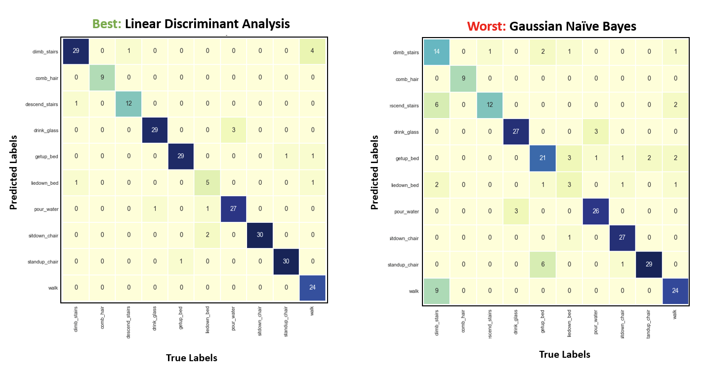
liedown_bed seems to be the most difficult activity to classify correctly: it is worth to note that it is also the class having the smallest support (see above), therefore if I were the Principal Investigator, I would recommend increase the number of liedown_bed recordings (as well as comb_hair and descend_stairs) so to balance all classes 😉
12. Build an ensemble classifier stacking the best classifiers
Except for the Gaussian Naive Bayes, all other classifiers perform pretty well, so I will keep all except GaussianNB to build an ensemble classifier. One nice feat of sklearn's StackingClassifiers() class is that it automatically performs cross-validation on the estimators (see my post on Model Validation), so that the resulting final performance should be more robust as it controls for possible over-fitting.

Wow, F1-score of ~0.92 is really not bad as performance for a naif approach!
USING tsfresh

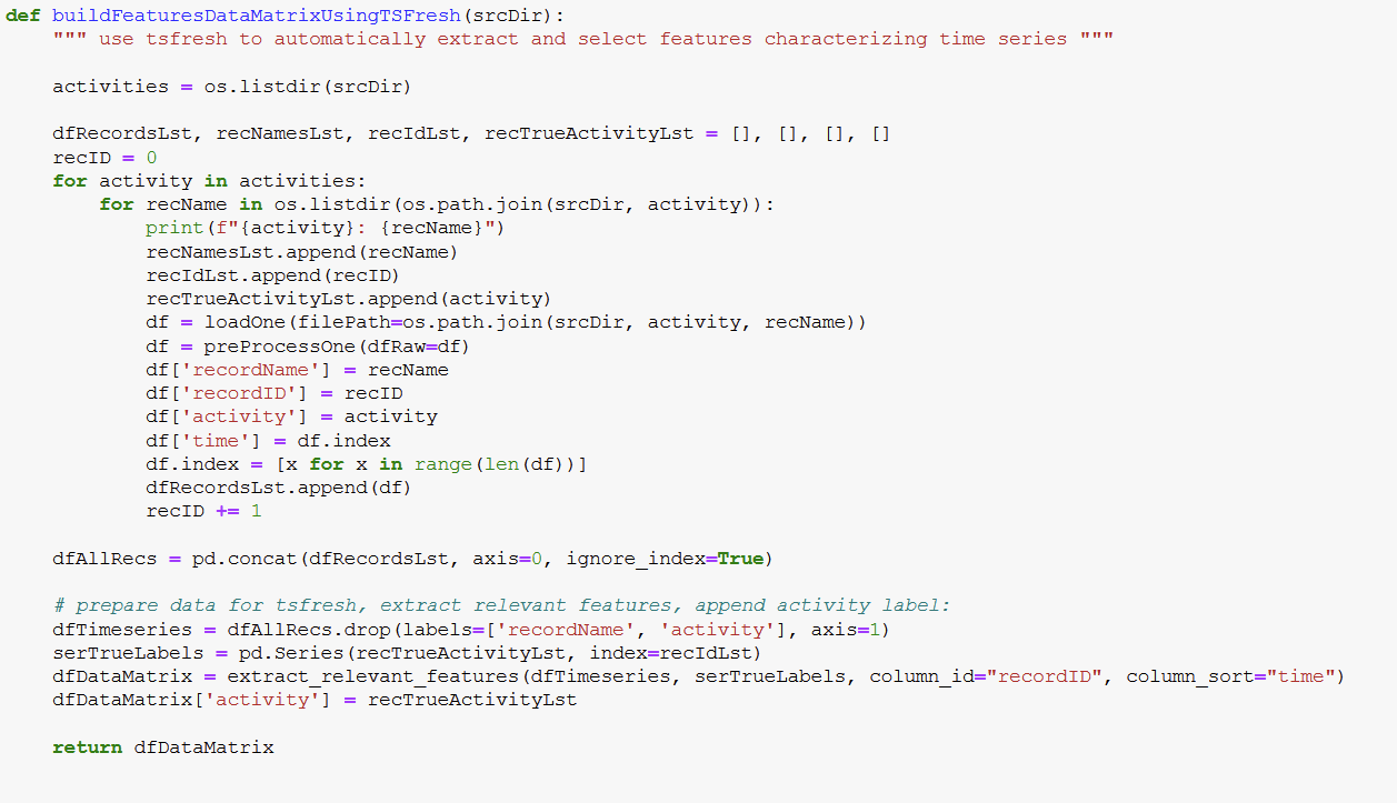


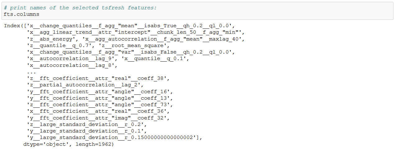
tsfresh automatically selects 1962 features as relevant 😮 Let's print their names to have an idea of which those features are:

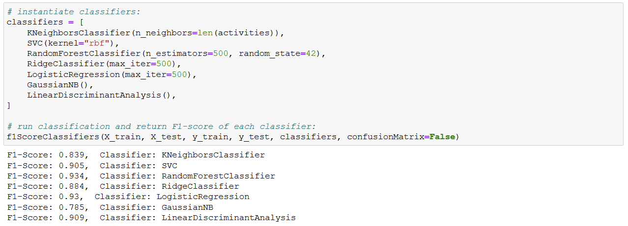

As we can see, using tsfresh-derived features we get even better results!
